Introduction to the Jupyter Notebook
The Jupyter notebook is a browser based scientific notebook, and is, therefore, extremely useful for learning and doing data science tasks. While Jupyter initially supported the Python programming language, via the IPython kernel, Jupyter now supports many additional programming languages, including R, Julia, and Haskell. In addition, you can directly embed scripts, including Bash shell scripts, within a cell. This technology has gained tremendous popularity quite rapidly, and is continuing to be developed as Project Jupyter, which highlights the programming language agnostic view the notebook concept has embraced. In addition, the Jupyter team develops and maintains a set of Docker images to simplify the adoption of notebooks.
In this notebook, we will explore the Jupyter Notebook, specifically focusing on
- Magics
- Writing markdown formatted cells
- Including math formulae
- Writing and executing Python code
- Visualizing plots
- Writing and executing Unix commands
- Writing and executing Bash shell scripts
Our coverage of most of these topics will be brief, and given the time limitations of this course, some topics will be covered in more detail in subsequent lessons. For some topics, links will be provided for more detailed reference; a good example is Jupyter's Rich Output capabilities. However, we will explore some topics, such as writing and executing code, in more detail through the rest of this course.
The Jupyter team has provided a nice introduction to working in an IPython Notebook, including how to use the menu commands, toolbar, and keyboard shortcuts. Of these, the most important points are to use the mouse to select a cell by single-clicking, and to enter a cell for editing by double-clicking. To have the IPython kernel process a cell, you can either enter control-return, which processes and remains in the current cell, or shift-return, which processes the cell and advances to the next cell. Finally, another important keyboard trick is to place a question mark, ?, at the end of a IPython magic or Python keyword to bring up an IPython message window that provides online details for the magic or keyword.
Magics
Jupyter provides specific commands, known as magics, that you can execute within a code cell to provide enhanced functionality to the current notebook. Magics are not part of the Python programming language, but can often make programming easier, especially within the notebook, and some magics can be used to improve your data processing work flow. Magics come in two types:
- line magics, and
- cell magics.
To see the list of currently available magics, execute the following cell.
%lsmagic
Line magic
A line magic is prepended by a single % character, and will have any arguments specified all on the same line. As a caveat to this statement, if the line magic Automagic is set to on, the preceding `%
character is not required. Some useful line magics include:
%lsmagic, which lists all currently defined line and cell magics for the current notebook,%matplotlib, which allows inline plotting to be enabled (and is preferred over the old%pylabmagic,%run, which will run the named file as a program in the current cell,%autosave, which sets the default autosave frequency in seconds, and%timeit, which in line mode times the execution of a single line of code.
Cell magics
A cell magic is prepended by two % characters, and they can have arguments that include both the current line and the remaining lines in the current cell. Thus, cell magics must be placed on the first line of a cell, and in general you can only have one cell magic per cell. Some useful line magics include:
- '%%timeit', which can be used to time a multi-line Python statement,
- '%%run',
- '%%writefile' writes the contents of the cell into the named file,
- '%%script', which can be used to create and run a script in a subprocess including Python, Bash, or R, and
- '%%bash', which lets you run a Bash shell script and optionally capture the STDOUT and STDERR streams into variables.
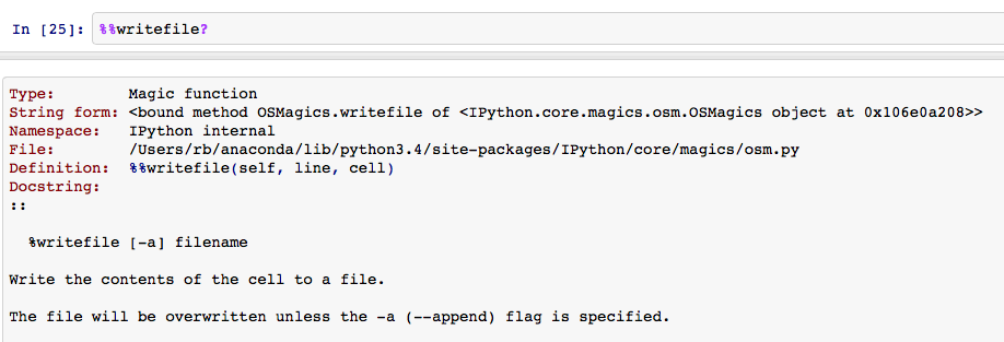
If you are uncertain how to use a particular magic, you can always obtain help from the IPython kernel by entering the magic by itself in a cell, adding a ? character at the end, and executing the cell to bring up the IPython help window, as shown below for the %%writefile magic.
Header Cells
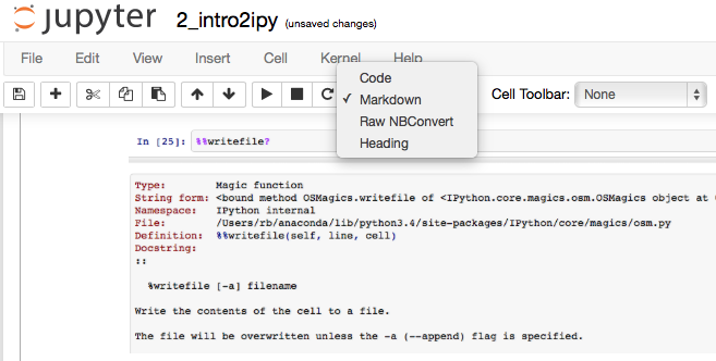
While you can use Markdown, described next, to create formatted header lines, the recommended technique is to explicitly make a header cell. You can create a cell to hold the header text, for example "Introduction to the Jupyter Notebook" and change the cell type to the appropriate header level by using the cell toolbar, as shown below.
Raw NBConvert Cells
The IPython Notebook can be converted into a number of different output formats. The nbconvert tool is used to convert from the default JSON native format of an ipynb file into the desired output format. The contents of any Raw NBConvert cell are left unmodified during output. This allows for post-processing of the generated file, such as with LaTeX or Restructured Text. These cells are beyond the scope of this course.
Markdown Cells
Markdown is a plain text formatting syntax that you can easily use to write text that can be converted to formatted text, for example, HTML. Markdown was developed by John Gruber, who runs the popular Daring Fireball blog. Markdown has found many uses, two of which are relevant for this course:
- github documentation pages, and
- IPython notebook documentation cells.
Markdown is free software that is available under a BSD—style open source license. Markdown will be covered in more detail in a subsequent lesson.
Unix Commands
Later in this course, we will discuss how to explore the Unix file system at the Unix command line. We can actually execute nearly all of these commands from within the IPython Notebook by using a Code Cell and preceding the Unix command by an exclamation point. For example, to display the current working directory, we would enter !pwd and subsequently execute this code cell.
This capability is actually very useful; for example, we can put a wget command at the start of an IPython Notebook to retrieve a data set that will be used in the rest of the notebook. This makes the notebook self-contained and easy to share or distribute to run in a Docker container on another machine. This sequence can be seen in the following figure:
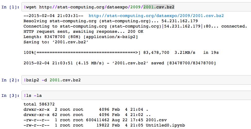
If you try a complex command, like the wget example, in your Jupyter Notebook, you will also see the non-blocking capability of an IPython Code Cell, since the Unix command runs in the background allowing you to continue working within the Notebook. Working with the Unix filesystem will be covered in more detail in a subsequent lesson.
Writing and Executing Code
Of course, the reason we are using IPython Notebooks is that they allow for in place development and execution of Python code. There are a number of direct benefits you accrue by developing and executing code in an IPython Notebook:
- Run code in place with the output displayed in the notebook,
- Display visualizations inline,
- Run code in the background, while you edit or run code in other cells,
- Clean restarts of the IPython kernel, and
- Built-in support for parallelization.
The simplest of these capabilities to demonstrate is developing and running code in the Notebook. The code can be a single line or multiple lines. Code cells can be executed by using one of two key combinations: CONTROL-return, which executes the cell in place, or SHIFT-return, which executes the code and advances to the next cell. For example, as shown below, we have a single line of Python code that can be executed with the output directly shown.
print("Hello World!")
Python Programs
A Jupyter Notebook code cell can take a full Python program, including importing Python libraries, which are in scope for the remainder of the Notebook. For example, we can compute the integral shown earlier by importing a constant and a function from the numpy library and an integration function from the scipy library:
$\int_0^{\pi} \sin(\theta)\ d\theta = 2$
Note: At this point you are not expected to understand the Python statements being demonstrated. They are only being used for demonstration purposes and will be introduced more completely later in this course.
import numpy as np
from scipy.integrate import quad

print("The Integral = %3.1f" % quad(np.sin, -2.0 * np.pi, np.pi)[0])
Inline Figures
When making data visualization, the resulting plots or images can be displayed inline. The recommended way to accomplish this is to use the %matplotlib line magic, which will inform the IPython kernel to display the image inline; this magic can take either the inline or the notebook value; the inline value will generally be preferred in this class for simplicity. Note that you may see suggestions to use the %pylab line magic, but this approach is no longer recommended since it pollutes the global namespace by importing several Python libraries.
%matplotlib inline

theta = np.arange(0., np.pi, 0.01)
y = np.sin(theta)

import matplotlib.pyplot as plt

plt.plot(theta, y)
plt.xlabel(r"$\theta$")
plt.ylabel(r"$\sin$($\theta$)")
plt.title("My Awesome Title")
plt.show()

Running Code in the Background
One of the features of the IPython kernel used in a Jupyter notebook to run Python programs that novices fail to appreciate is the ability for code, by default, to run in the background. This is useful, as we will see throughout this course, both when developing, but also when executing code. For example, the following code block slowly prints out a series of numbers, by default the integers from 0 to 19. When we execute the cell, the integers slowly print out while we are free to edit or run code in other cells.
# First we handle our imports.
import sys
from time import sleep

# Parameters that we can change
s = 20
t = 2

# Now loop, printing out a new number before sleeping
for i in range(s):
    sys.stdout.write("%3d," % i)
    sys.stdout.flush()
    sleep(t)

# The code continues to run in the background
Clean Kernel Restarts
In some occasions, our code might cause the Python interpreter to crash. While this normally might be a serious concern, the IPython kernel can detect this condition and initiate a clean restart. In this Notebook, we won't intentionally do this; however, you may experience a kernel crash when working on assignments or projects in this course.
Ancillary Information
The following links are to additional documentation that you might find helpful in learning this material. Reading these web-accessible documents is completely optional.
- Project Jupyter
- Demonstration Jupyter Notebook
- Jupyter Documentation
- IPython Documentation
© 2017: Robert J. Brunner at the University of Illinois.
This notebook is released under the Creative Commons license CC BY-NC-SA 4.0. Any reproduction, adaptation, distribution, dissemination or making available of this notebook for commercial use is not allowed unless authorized in writing by the copyright holder.